

If you run an industrial treatment plant, you already know the hardest part isn’t building the system — it’s keeping it stable when the feed changes every day. That’s where optimization software has quietly become one of the most practical tools we have. In my experience commissioning evaporators, membrane trains, and dewatering lines, the plants that hold their setpoints through a production upset are the ones running some form of model-based control or predictive monitoring. This article walks through where these tools actually earn their keep, where they don’t, and how to think about the engineering trade-offs before you buy anything.
Why Industrial Wastewater Is Hard to Optimize in the First Place
Municipal plants see slow, seasonal shifts. Industrial plants see step changes. A plating line dumps a rinse batch, a pharmaceutical campaign switches solvents, a landfill cell gets three inches of rain. Conductivity, COD, oil content, and pH can move within hours.
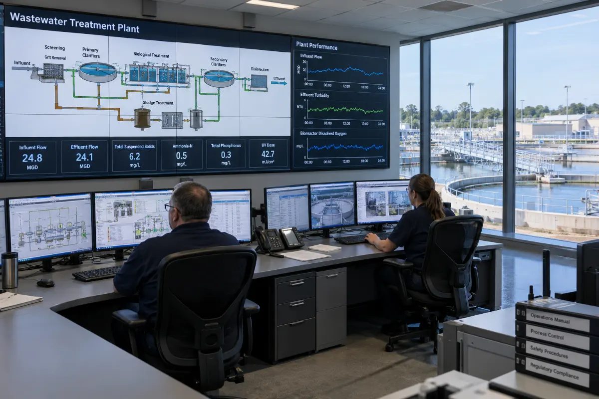
Classical control loops handle this poorly because they react after the fact. A PID controller on evaporator density only knows the outlet is already too concentrated. By then you’ve fouled a heat exchanger surface or tripped a compressor on high discharge temperature.
What optimization software gives you is a forward-looking layer. Instead of reacting to a measurement, it predicts where the process is heading and trims the setpoints before the excursion happens. That’s the whole value proposition, and everything else is detail.

The Layers of a Practical Optimization Stack
Vendors love to sell this as one big black box. In reality, a working system has four distinct layers, and each one fails in its own way.
| Layer | What it does | Typical failure mode |
|---|---|---|
| Instrumentation & data acquisition | Reads flow, conductivity, pH, turbidity, pressure, temperature, power draw | Drifting sensors, fouled probes, missing tags |
| Soft sensors / virtual analyzers | Estimates values you can’t measure online (COD, scaling potential, oil content) | Model drift after feed composition changes |
| Predictive models | Forecasts fouling rate, membrane flux decline, evaporator scaling | Overfitting to a narrow historical dataset |
| Advisory or closed-loop control | Adjusts dosing, blowdown, feed rate, CIP scheduling | Operator distrust; alarms ignored |
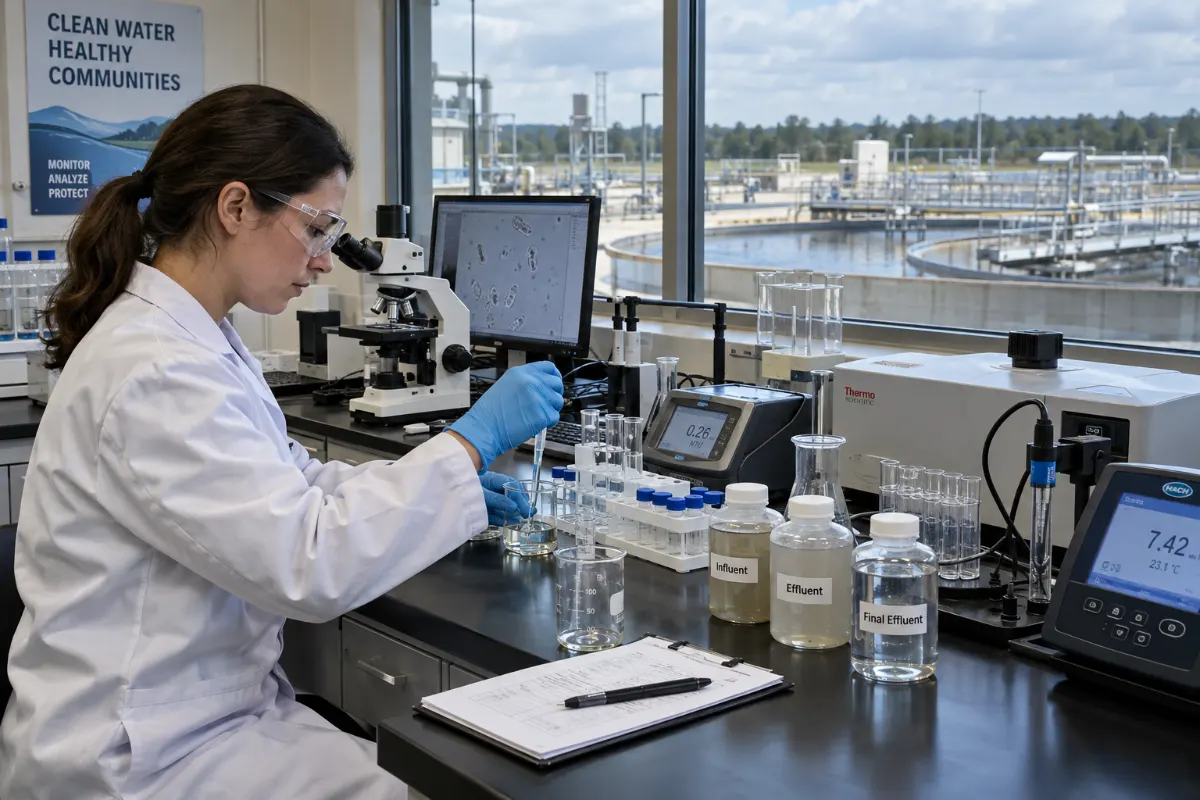
Notice that three of the four layers are not really about algorithms. They’re about measurement quality and process understanding. If your conductivity probe is reading 15% high, no model in the world will save you.
Where Optimization Actually Pays Off: Five Concrete Applications
1. Chemical Dosing and Coagulant Control
This is usually the fastest payback. Coagulant and polymer dosing in a dissolved air flotation or clarification stage is often run on a fixed flow-proportional setpoint because operators can’t measure the right thing in real time. A soft sensor built on turbidity, streaming current, and jar-test history can trim dosing by a meaningful margin without risking effluent quality.
Typical design range: 10–25% reduction in coagulant consumption at plants that were previously running conservative fixed doses. Your number depends on how much safety margin you were carrying to begin with.
2. Evaporator and MVR Stability
Mechanical vapor compression and multi-effect systems are unforgiving. A 2°C rise in boiling point elevation can push a compressor toward its surge line. Optimization here means predicting the boiling point from feed conductivity and density, then trimming the circulation rate and discharge setpoint accordingly.
On a recent landfill leachate project, this kind of feed-forward control cut the number of high-temperature trips from roughly weekly to almost never. The hardware didn’t change — only the control logic did. If you want to understand the equipment side first, it’s worth reviewing how mechanical vapor compression evaporators are structured before designing control around them.
3. Membrane Fouling and Cleaning Schedules
Reverse osmosis and DTRO trains are usually cleaned on a calendar, not on condition. That means you either clean too often (wasting chemicals and membrane life) or too late (irreversible fouling).
A pressure-drop and normalized-flux model can predict when the next cleaning is actually due. In practice, plants using condition-based cleaning on DTRO membrane systems often extend cleaning intervals by 20–40% on stable feeds, though high-fouling streams see less benefit.
4. Sludge Dewatering Optimization
Screw press and centrifuge performance depends on feed solids, polymer dose, and torque. Optimizing polymer dose against cake dryness in real time is a classic application — and one of the easiest to justify because polymer is expensive.
Typical indicative range: 15–30% polymer savings with cake dryness held within ±2 percentage points. Again, project-dependent.
5. Energy and Load Shifting
Evaporators and high-pressure pumps are the biggest electrical loads on most industrial wastewater sites. If your utility offers time-of-use rates, shifting thermal or hydraulic buffer capacity to off-peak hours can reduce energy cost even when total kWh stays flat.
Where These Systems Fail — and Why
I’ve seen more optimization projects fail for non-technical reasons than technical ones. The pattern is consistent:
- No baseline data. If you can’t describe how the plant performed for the last six months, you can’t prove improvement.
- Unreliable instruments. A model fed by a drifting pH probe is worse than no model.
- Operators not involved. If the advisory system says “reduce feed by 8%” and nobody knows why, they’ll override it.
- Scope creep. Trying to optimize the entire plant in one phase instead of one unit operation at a time.
- No maintenance plan for the model itself. Models drift. Someone has to own them.
“The best optimization project I’ve been part of started with three months of instrument calibration and data cleanup before a single line of control logic was written. That’s not glamorous, but it’s what made the rest work.” — a commissioning engineer I’ve worked with for years
How to Choose Between Advisory and Closed-Loop Control
This is the single biggest decision in the design phase, and it’s usually made badly.
| Factor | Advisory system | Closed-loop control |
|---|---|---|
| Operator trust required | Low to moderate | High — must be earned over months |
| Instrumentation quality needed | Moderate | High; redundancy often required |
| Payback speed | Slower — depends on operator adoption | Faster once validated |
| Risk if model is wrong | Low — human in the loop | High — needs hard interlocks |
| Best fit | Complex, variable, or poorly instrumented processes | Stable processes with good sensors and clear economics |
My rule of thumb: start advisory, run it for six months, and only close the loop on the two or three variables where the operators already agree with the recommendations. Everything else stays advisory.
Instrumentation: The Part Everyone Underestimates
You cannot optimize what you cannot measure. Before any software project, budget for:
- Redundant conductivity and pH on critical streams
- Online turbidity or suspended solids where dosing is controlled
- Pressure and temperature transmitters on every heat exchanger and membrane stage
- Power monitoring on the largest motors
- A historian that actually stores high-resolution data, not 15-minute averages
On a typical mid-size industrial plant, instrumentation upgrades run 15–30% of the total optimization project cost. Skipping them is the most common reason projects underdeliver.
Energy, Cost, and Lifecycle Thinking
Optimization rarely changes the fundamental energy demand of a process. An MVR evaporator needs a certain specific energy per kilogram of water evaporated, and no control logic changes thermodynamics.
What optimization does change:
- Chemical consumption — usually the clearest win
- Cleaning frequency and downtime — often underestimated
- Equipment life — fewer thermal cycles, fewer fouling events
- Off-spec events — fewer permit exceedances, fewer emergency responses
- Operator time — fewer manual adjustments per shift
When you build the business case, put a number on all five. The chemical savings alone rarely justify the project; the combination usually does.
If you’re evaluating a zero liquid discharge or high-recovery configuration, the optimization layer is often what makes the difference between a system that runs at design capacity and one that limps along at 70%. It’s worth reviewing how zero liquid discharge systems are typically structured before deciding where to apply control.
Case-Style Analysis: Three Anonymous Scenarios
Electroplating Rinse Water Recovery
A plating shop with a high-recovery RO and evaporator train was running manual blowdown based on a daily lab sample. Feed conductivity varied with production schedule. After adding a soft sensor for scaling potential and automated blowdown control, the plant reduced cleaning frequency substantially and stabilized distillate quality. No new membranes were added.
Pharmaceutical Batch Wastewater
Campaign-based production meant the feed changed every few days. Optimization focused on early detection of solvent surges using a combination of COD analyzer trends and evaporator pressure signals. Operators received an advisory alert 30–60 minutes before a trip would have occurred. The main benefit was fewer unplanned shutdowns, not energy savings.
Landfill Leachate Treatment
Leachate composition shifts seasonally and after rainfall. A predictive model on the biological stage helped adjust aeration and carbon dosing ahead of load spikes. The plant maintained discharge compliance through wet-weather events that had previously caused excursions.
These are indicative scenarios drawn from common project patterns, not specific client results. Your numbers will depend on feed variability, instrumentation quality, and how much of the process is already automated.
Implementation Roadmap That Actually Works
- Baseline. Six months of clean historical data on the target unit operation.
- Instrument audit. Calibrate, replace, or add what’s missing. Don’t skip this.
- Soft sensors. Build and validate virtual measurements before any control logic.
- Advisory mode. Run recommendations alongside operators for 3–6 months.
- Closed-loop on selected loops. Only where operators trust the output and hard interlocks exist.
- Model maintenance. Assign ownership, schedule retraining, monitor drift.
Most plants should expect 9–18 months from kickoff to a stable closed-loop system on two or three loops. Anything faster usually means corners were cut.
Common Operational Problems and What They Usually Mean
| Symptom | Likely cause | First check |
|---|---|---|
| Model recommendations drift over weeks | Sensor calibration or feed composition shift | Compare lab results to online readings |
| Operators ignore alerts | Too many false positives | Review alert thresholds and deadbands |
| Savings disappear after 6 months | No model maintenance | Check retraining schedule |
| Control loop oscillates | Model too aggressive for process dynamics | Increase deadband or switch to advisory |
| Instrumentation fails frequently | Wrong sensor for the stream | Review material compatibility and cleaning method |
Engineering Advice Before You Commit
Three things I tell every client before they sign an optimization contract:
- Fix the process first. If your evaporator is undersized or your membranes are at end of life, optimization won’t help. Solve the physical problem.
- Start with one unit operation. Not the whole plant. Prove the concept, then expand.
- Own the data. Make sure you have full access to your historian and model outputs. Vendor lock-in on data is a real risk.
Regulators and lenders increasingly expect documented process control and monitoring. The U.S. EPA’s National Pollutant Discharge Elimination System framework and the World Bank’s water resources guidance both emphasize continuous monitoring and adaptive management — which is exactly what a well-built optimization layer provides.
Planning an optimization project on an evaporator, membrane, or ZLD train? We’ve commissioned systems across plating, pharma, chemical, and leachate applications. Bring us your feed data and we’ll help you scope what’s realistic — and what isn’t.
FAQ
Do I need a full machine learning platform, or will rule-based control work?
For most industrial plants, rule-based control combined with a good soft sensor gets you 70–80% of the benefit. Full model-based control makes sense when the process is complex, the feed is highly variable, and the economics justify the extra engineering. Start simple.
How much does an optimization project typically cost?
For a single unit operation, expect instrumentation and controls to run a significant fraction of the total cost, with software and engineering on top. Project-dependent, but budget at least a few months of engineering time plus hardware. The payback usually comes from chemicals, downtime, and off-spec reduction combined.
Can I retrofit optimization onto an existing plant?
Yes, and most projects are retrofits. The constraint is usually instrumentation — older plants often lack the sensors needed. The retrofit itself is straightforward once the measurement layer is in place.
How do I know if the model is still accurate six months later?
Track a small set of key performance indicators against lab results weekly. If the gap between predicted and measured values grows beyond your tolerance, retrain or recalibrate. Assign one person to own this.
What’s the biggest mistake plants make?
Buying software before fixing instrumentation. If your sensors are drifting, no model will help. Fix the measurement layer first, then optimize.
Will this help me meet tighter discharge limits?
It helps you stay consistent, which matters more than peak performance. Fewer excursions means fewer permit issues. But if your treatment train is fundamentally undersized, optimization won’t close the gap — you need process upgrades.
Does it work on membrane systems like RO and DTRO?
Yes, and this is one of the strongest applications. Predicting normalized flux decline and cleaning timing is well understood and delivers measurable results on most industrial RO and DTRO trains.
How long until I see results?
Advisory mode typically shows value within 3–6 months. Closed-loop control takes longer because you need operator trust and validation. Plan for 9–18 months to a mature system.